写在前面:大家好!我是【AI 菌】,一枚爱弹吉他的程序员。我
热爱AI、热爱分享、热爱开源
! 这博客是我对学习的一点总结与记录。如果您也对
深度学习、机器视觉、算法、Python、C++
感兴趣,可以关注我的动态,我们一起学习,一起进步~
【AI 菌】的博客
【AI 菌】的Github
一、回归问题
回归问题在生活中是很常见的,比如股价的走势预测、天气预报中温度和湿度等的预测、交通流量的预测等。对于预测值是连续的实数范围,或者属于某一段连续的实数区间的问题称为
回归问题
,回归问题是一种连续值预测问题。
特别地,如果使用线性模型去逼近真实模型,那么我们把这一类方法叫做
线性回归
(Linear Regression,简称 LR),线性回归是回归问题中的一种具体的实现。
二、问题描述
我们有一个数据集,这个数据集中包含100个已知点(x, y)。我们希望,建立一个数学模型,对于任意的新输入x,该模型都能输出一个近似于真实值的结果。
如果我们换一个角度来看待这个问题,它其实可以理解为一组连续值的预测问题。给定数据集𝔻,我们需要从𝔻中学习到数据的真实模型,从而预测未见过的样本的输出值。
在假定模型的类型后,学习过程就变成了搜索模型参数的问题,比如我们假设神经元为线性模型,那么训练过程即为搜索线性模型的𝒘和𝑏参数的过程。训练完成后,利用学到的模型,对于任意的新输入𝒙,我们就可以使用学习模型输出值作为真实值的近似。
为了使模型尽可能地简单,我们假定该线性模型为一次函数
y = wx + b
三、模型搭建与训练
完整代码已经上传我的Github仓库,欢迎star:
https://github.com/Keyird/TensorFlow2-for-beginner
(1) 数据准备及可视化
本次数据集一共包含100个坐标点(x, y),在data.csv文件中直接给出。部分数据如下所示:
points = np. genfromtxt( "data.csv" , delimiter= "," )
为了更直观地感受,下面使用matplotlib对这些点进行可视化:
plt. scatter( points[ : , 0 ] , points[ : , 1 ] )
x = np. arange( 0 , 100 )
y = w * x + b
plt. xlabel( 'x' )
plt. ylabel( 'y' )
plt. show( )
这100个点的分布如下图所示:
(2) 计算梯度、更新权值
在计算梯度前,我们需要先确定损失函数。本次实验我们采用简单的
平方和误差
作为损失函数:
l
o
s
s
=
∑
i
(
w
x
i
+
b
−
y
i
)
2
loss=\sum_i(wx_i +b -y_i)^2
l
o
s
s
=
∑
i
(
w
x
i
+
b
−
y
i
)
2
根据梯度下降法,可以推知权值w、b的更新公式:
w
′
=
w
−
l
r
∗
σ
l
o
s
s
σ
w
w^{'} = w-lr * \frac{\sigma loss}{\sigma w}
w
′
=
w
−
l
r
∗
σ
w
σ
l
o
s
s
b
′
=
b
−
l
r
∗
σ
l
o
s
s
σ
b
b^{'} = b-lr * \frac{\sigma loss}{\sigma b}
b
′
=
b
−
l
r
∗
σ
b
σ
l
o
s
s
,其中
l
r
lr
l
r
为学习率
对参数w、b分别求偏倒可得:
σ
l
o
s
s
σ
w
=
2
∑
(
w
x
i
+
b
−
y
i
)
x
i
\frac{\sigma loss}{\sigma w}=2\sum(wx_i +b -y_i)x_i
σ
w
σ
l
o
s
s
=
2
∑
(
w
x
i
+
b
−
y
i
)
x
i
σ
l
o
s
s
σ
b
=
2
∑
(
w
x
i
+
b
−
y
i
)
\frac{\sigma loss}{\sigma b}=2\sum(wx_i +b -y_i)
σ
b
σ
l
o
s
s
=
2
∑
(
w
x
i
+
b
−
y
i
)
注:由于偏导符号不会打,所以以上式子中的偏导符号均由
σ
\sigma
σ
符号代替。
在训练过程中,一次输入100组数据,计算平均梯度,对当前轮的参数w、b进行更新:
def step_gradient ( b_current, w_current, points, learningRate) :
b_gradient = 0
w_gradient = 0
N = float ( len ( points) )
for i in range ( 0 , len ( points) ) :
x = points[ i, 0 ]
y = points[ i, 1 ]
b_gradient += ( 2 / N) * ( ( w_current * x + b_current) - y)
w_gradient += ( 2 / N) * x * ( ( w_current * x + b_current) - y)
new_b = b_current - ( learningRate * b_gradient)
new_w = w_current - ( learningRate * w_gradient)
return [ new_b, new_w]
1 2 3 4 5 6 7 8 9 10 11 12 13 14 15 16 17 18 1 2 3 4 5 6 7 8 9 10 11 12 13 14 15 16 17 18
(3) 设置初始值
learning_rate = 0.0001
initial_b = 0
initial_w = 0
num_iterations = 1000
(4) 迭代训练指定次数
以initial_b, initial_w为初始权值,learning_rate为学习率,迭代训练num_iterations次
def gradient_descent_runner ( points, starting_b, starting_w, learning_rate, num_iterations) :
b = starting_b
w = starting_w
for i in range ( num_iterations) :
b, w = step_gradient( b, w, np. array( points) , learning_rate)
return [ b, w]
[ b, w] = gradient_descent_runner( points, initial_b, initial_w, learning_rate, num_iterations)
四、实验结果与预测
(1) 训练前后损失对比
将100组数据的平均损失作为损失进行计算。
def compute_error_for_line_given_points ( b, w, points) :
totalError = 0
for i in range ( 0 , len ( points) ) :
x = points[ i, 0 ]
y = points[ i, 1 ]
totalError += ( y - ( w * x + b) ) ** 2
return totalError / float ( len ( points) )
分别计算训练前和训练后的平均损失,来进行比较:
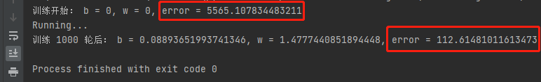
print ( "训练开始: b = {0}, w = {1}, error = {2}"
. format ( initial_b, initial_w, compute_error_for_line_given_points( initial_b, initial_w, points) ) )
print ( "Running..." )
[ b, w] = gradient_descent_runner( points, initial_b, initial_w, learning_rate, num_iterations)
print ( "训练 {0} 轮后: b = {1}, w = {2}, error = {3}" .
format ( num_iterations, b, w, compute_error_for_line_given_points( b, w, points) ) )
输出对比:
(2) 可视化拟合结果
通过matplotlib绘制拟合结果:
plt. scatter( points[ : , 0 ] , points[ : , 1 ] )
x = np. arange( 0 , 100 )
y = w * x + b
plt. xlabel( 'x' )
plt. ylabel( 'y' )
plt. title( "y = wx + b" )
plt. plot( x, y, color= 'r' , linewidth= 2.5 )
plt. show( )
直线拟合结果如下:
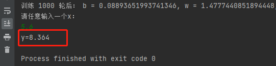
(3) 输入任意x,预测y值
通过1000次迭代训练,我们已经得到了优化后的w,b,即直线。因此当我们任意输入一个新的x,可以根据拟合好的直线y=1.4777x+0.0889,得到预测值y。
print ( "请任意输入一个x:" )
x = eval ( input ( ) )
print ( "y={:.3f}" . format ( w* x+ b) )
如下图所示,当我们随便输入一个x=5.6,经过线性回归,预测得到y=8.364。
本教程所有代码会逐渐上传github仓库:
https://github.com/Keyird/TensorFlow2-for-beginner
由于水平有限,博客中难免会有一些错误,有纰漏之处恳请各位大佬不吝赐教!
推荐文章
最好的关系是
互相成就
,各位的「三连」就是【AI 菌】创作的最大动力,我们下期见!